1 Introduction
The practice of measuring phenomena by having one or more raters assign to items one of a set of ratings is common across many fields. For example, in medicine one or more doctors may classify a diagnostic image as being evidence for one of several diagnoses, such as types of cancer. This process of rating is often done by one or more expert raters, but may also be performed by a large group of non-experts (e.g., in natural language processing (NLP), where a large number of crowd-sourced raters are used to classify pieces of text; see Passonneau and Carpenter (2014) and Ipeirotis et al. (2010)) or by a machine or other automated process (e.g., a laboratory diagnostic test, where ‘test’ may refer to either the raters and/or the ratings). Other fields where ratings occur include astronomy, for classifying astronomical images (Smyth et al. 1994), and bioinformatics, for inferring error rates for some bioinformatics algorithms (Jakobsdottir and Weeks 2007). Indeed, both studies apply the Dawid–Skene model that we present below and implement in our software package.
The assignment of items to categories, which are variously referred to as gradings, annotations or labelled data, we will call ratings. Our hope is that these are an accurate reflection of the true characteristics of the items being rated. However, this is not guaranteed; all raters and rating systems are fallible. We would expect some disagreement between the raters, especially from non-experts, and even expert raters may disagree when there are some items that are more difficult to rate than others. A typical way of dealing with this problem is to obtain multiple ratings for each item from different raters, some of whom might rate the item more than once on separate occasions. By using an aggregate index (e.g., by averaging the ratings) one can hope to reduce bias and variance when estimating both population frequencies and individual item categories.
Despite the fact that ratings data of this type are common, there are few software packages that can be used to fit useful statistical models to them. To address this, we introduce rater, a software package for R (R Core Team 2021) designed specifically for such data and available on CRAN. Our package provides the ability to fit the Dawid–Skene model (Dawid and Skene 1979) and several of its extensions. The goal is to estimate accurately the underlying true class of each item (to the extent that this is meaningful and well-defined) as well as to quantify and characterise the accuracy of each rater. Models of these data should account for the possibility that accuracy differs between the raters and that the errors they make might be class-specific. The package accepts data in multiple formats and provides functions for extracting and visualizing parameter estimates.
While our package implements optimisation-based inference, the default mode of inference is Bayesian, using Markov Chain Monte Carlo (MCMC). We chose a Bayesian approach for several reasons. The first is because the standard classical approach, using an EM algorithm, often gives parameter estimates on the boundary of the parameter space (i.e., probabilities of exactly 0 or 1), which would typically be implausible. Examples of this can be seen in the original paper by Dawid and Skene (1979), and also in our own results below that compare MCMC and optimisation-based inference (e.g., compare Figure 2 and Figure 4). A second reason is to take advantage of the convenient and powerful Stan software (Stan Development Team 2021), which made implementing our package considerably easier. Stan is a probabilistic programming language that implements MCMC and optimisation algorithms for fitting Bayesian models. The primary inference algorithm used by Stan is the No U-Turn Sampler (NUTS) variant of the Hamiltonian Monte Carlo (HMC) sampler, which uses gradient information to guide exploration of the posterior distribution. A third reason is that it allows users to easily incorporate any prior information when it is available. In this context, prior information might be information about the quality of the raters or specific ratings mistakes that are more common.
We illustrate our methods and software using two examples where the raters are healthcare practitioners: one with anaesthetists rating the health of patients, and another with dentists assessing the health of teeth. In both examples, we are interested in obtaining more accurate health assessments by combining all of the experts’ ratings rather than using the ratings of a single expert, as well as estimating the accuracy of each expert and characterising the types of errors they make.
Our paper is organised as follows. Section 2 describes the various data formats that can be used with the function implemented in the package. Section 4 introduces the Dawid–Skene model and several of its extensions. Section 5 briefly describes the implementation and goes into more detail about some of the more interesting aspects, followed by an exposition of the technique called Rao–Blackwellization in Section 6, which is connected with many aspects of the implementation. Section 7 introduces the user interface of rater along with some examples. Section 8 concludes with a discussion of the potential uses of the model.
2 Data formats
There are several different formats in which categorical rating data can be expressed. We make a distinction between balanced and unbalanced data. Balanced data have each item rated at least once by each rater. Unbalanced data contain information on some items that were not rated by every rater; stated alternatively, there is at least one rater who does not rate every item.
Table 1 and Table 2 illustrate three different formats for categorical rating data. Format (a) has one row per item-rater rating episode. It requires variables (data fields) to identify the item, the rater and the rating. This presentation of data is often referred to as the ‘long’ format. It is possible for a rater to rate a given item multiple times; each such rating would have its own row in this format. Format (b) has one row per item, and one column per rater, with each cell being a single rating. Format (c) aggregates rows (items) that have identical rating patterns and records a frequency tally. Formats (b) and (c) are examples of ‘wide’ formats. They only make sense for data where each rater rates each item at most once. Note that the long format will never require any structural missing values for any of the variables, whereas the wide formats require the use of a missing value indicator unless they represent data generated by a balanced design, see Table 2. One benefit of the grouped format is that it allows a more computationally efficient implementation of the likelihood function. See Section 5 for details about how this is implemented in rater.
|
|
|
|
|
|
3 Existing approaches
A typical approach for modelling categorical ratings is to posit an unobserved underlying true class for each item, i.e., we represent the true class as a latent variable. One of the first such models was developed by Dawid and Skene (1979). This model is still studied and used to this day, and has served as a foundation for several extensions (e.g., Paun et al. 2018). Our R package, rater, is the first one specifically designed to provide inference for the Dawid–Skene model and its variants.
The Python library pyanno (Berkes et al. 2011) also implements a Bayesian version of the Dawid–Skene model in addition to the models described by Rzhetsky (2009). However, unlike rater, pyanno only supports parameter estimation via optimisation rather than MCMC; i.e., it will only compute posterior modes rather than provide samples from the full posterior distribution. In addition, pyanno does not support variants of the Dawid–Skene model nor the support for grouped data implemented in rater.
More broadly, many different so-called ‘latent class’ models have been developed and implemented in software, for a wide diversity of applications (e.g., Goodman 1974). A key aspect of the categorical ratings context is that we assume our categories are known ahead of time, i.e., the possible values for the latent classes are fixed. The Dawid–Skene model has this constraint built-in, whereas other latent class models are better tailored to other scenarios. Nevertheless, many of these models are closely related and are implemented as R packages.
Of most interest for categorical ratings analysis are the packages poLCA (Linzer and Lewis 2011), BayesLCA (White and Murphy 2014) and randomLCA (Beath 2017), all of which are capable of fitting limited versions of the Dawid–Skene model. We explore the relationship between different latent class models in more detail in Section 4.7. Briefly: randomLCA can fit the Dawid–Skene model only when the data uses binary categories, BayesLCA can only fit the homogeneous Dawid–Skene model, and poLCA can fit the Dawid–Skene model with an arbitrary number of categories but only supports wide data (where raters do not make repeated ratings on items). Neither poLCA nor randomLCA support fully Bayesian inference with MCMC, and none of the packages support fitting variants of the Dawid–Skene model (which are available in rater).
4 Models
One of the first statistical models proposed for categorical rating data was that of Dawid and Skene (1979). We describe this model below, extended to include prior distributions to allow for Bayesian inference. Recently, a number of direct extensions to the Dawid–Skene model have been proposed. We describe several of these below, most of which are implemented in rater. For ease of exposition, unless otherwise stated, all notation in this section will assume we are working with balanced data and where each item is rated exactly once by each rater, one exception is that we present the Dawid–Skene model for arbitrary data at the end of Section 4.1.
Assume we have \(I\) items (for example, images, people, etc.) and \(J\) raters, with each item presumed to belong to one of the \(K\) categories: we refer to this as its ‘true’ category and also as its latent class (since it is unobserved). Let \(y_{i, j} \in \{1, \dots, K\}\) be the rating for item \(i\) given by rater \(j\).
4.1 Dawid–Skene model
The model has two sets of parameters:
\(\pi_k\): the prevalence of category \(k\) in the population from which the items are sampled. \(\pi_k \in (0, 1)\) for \(k \in \{1, \dots, K\}\), with \(\sum_{k = 1}^K \pi_i = 1\). All classes have some non-zero probability of occurring. We collect all the \(\pi_k\) parameters together into a vector, \(\pi = (\pi_1, \dots, \pi_K)\).
\(\theta_{j, k, k'}\): the probability that rater \(j\) responds with class \(k'\) when rating an item of true class \(k\). Here, \(j \in \{1, \dots, J\}\) and \(k, k' \in \{1, 2, ..., K\}\). We will refer to the \(K \times K\) matrix \(\theta_{j, k, k'}\) for a given \(j\) as the error matrix for rater \(j\). We represent the \(k\)th row of this matrix as the vector \(\theta_{j, k} = \left(\theta_{j, k, 1}, \theta_{j, k, 2}, \dots, \theta_{j, k, K}\right)\): this shows how rater \(j\) responds to an item with true class \(k\), by rating it as being in class \(1, 2, \dots, K\), according to the respective probabilities.
The model also has the following set of latent variables:
- \(z_i\): the true class of item \(i\). \(z_i \in \{1 ..., K\}\) for \(i \in \{1, ..., I\}\).
Under the Bayesian perspective, the model parameters and latent variables are both unobserved random variables that define the joint probability distribution of the model. As such, inference on them is conducted in the same way. However, we make the distinction here to help clarify aspects of our implementation later on.
The model is defined by the following distributional assumptions: \[ \begin{aligned} z_i &\sim \textrm{Categorical}(\pi), \quad \forall i \in \{1, \dots, I\}, \\ y_{i, j} \mid z_i &\sim \textrm{Categorical}(\theta_{j, z_i}), \quad \forall i \in \{1, \dots, I\}, j \in \{1, \dots, J\}. \end{aligned} \] In words, the rating for item \(i\) given by rater \(j\) will follow the distribution specified by: the error matrix for rater \(j\), but taking only the row of that matrix that corresponds to the value of the latent variable for item \(i\) (the \(z_i\)th row).
We now have a fully specified model, which allows use of likelihood-based methods. The likelihood function for the observed data (the \(y_{i,j}\)s) is \[ \Pr(y \mid \theta, \pi) = \prod_{i = I}^{I} \left(\sum_{k = 1}^{K} \left(\pi_{k} \cdot \prod_{j = 1}^{J} \theta_{j, k, y_{i,j}}\right)\right). \tag{1} \]
Note that the unobserved latent variables, \(z = ({z}_{1}, {z}_{2}, \ldots, {z}_{I})\), do not appear because they are integrated out (via the sum over the categories \(k\)). Often it is useful to work with the complete data likelihood where the \(z\) have specific values, for example if implementing an EM algorithm (such as described by Dawid and Skene (1979)). The somewhat simpler likelihood function in that case is \[ \Pr(y, z \mid \theta, \pi) = \prod_{i = I}^{I} \left(\pi_{z_{i}} \cdot \prod_{j = 1}^{J} \theta_{j, z_{i}, y_{i,j}}\right). \] In our implementation we use the first version of the likelihood, which marginalises over \(z\) (see Section 5.1). We do this to avoid needing to sample from the posterior distribution of \(z\) using Stan, as the HMC sampling algorithm used by Stan requires gradients with respect to all parameters and gradients cannot be calculated for discrete parameters such as \(z\). Alternative Bayesian implementations, perhaps using Gibbs sampling approaches, could work with the second version of the likelihood and sample values of \(z\) directly.
To allow for Bayesian inference, we place weakly informative prior probability distributions on the parameters: \[ \begin{aligned} \pi &\sim \textrm{Dirichlet}(\alpha), \\ \theta_{j, k} &\sim \textrm{Dirichlet}(\beta_k). \end{aligned} \] The hyper-parameters defining these prior probability distributions are:
\(\alpha\): a vector of length \(K\) with all elements greater than 0
\(\beta\): a \(K \times K\) matrix with all elements greater than 0, with \(\beta_k\) referring to the \(k\)th row of this matrix.
We use the following default values for these hyper-parameters in rater: \(\alpha_k = 3\) for \(k \in \{1, \dots, K\}\), and \[ \beta_{k, k'} = \begin{cases} N p & \textrm{if } k = k' \\ \dfrac{N (1 - p)}{K - 1} & \textrm{otherwise} \end{cases} \quad \forall k, k' \in \{1, \dots, K\}. \] Here, \(N\) corresponds to an approximate pseudocount of hypothetical prior observations and \(p\) an approximate probability of a correct rating (applied uniformly across all raters and categories). This affords us the flexibility to centre the prior on a particular assumed accuracy (via \(p\)) as well as tune how informative the prior will be (via \(N\)). In rater we set the default values to be \(N = 8\) and \(p = 0.6\), reflecting a weakly held belief that the raters are have a better than coin-flip chance of choosing the correct class. This should be suitable for many datasets, where the number of categories is small, for example, less than ten. This default would, however, be optimistic if the number of categories is very large, for example, one hundred. In that case it would make sense for the user to specify a more realistic prior (see Section 7.5). A derivation of the default prior specification is shown in Section 4.2.
We can also write the Dawid–Skene model in notation that does not assume the data are balanced. Let \(I\), \(J\), \(K\) be as above. Let \(N\) be the total number of ratings in the dataset (previously we had the special case \(N = I \cdot J\)). Define the following quantities relating to the \(n\)th rating: it was performed by rater \(j_n\), who rated item \(i_n\), and the rating itself is \(y_n\). We can now write the Dawid–Skene model as: \[ \begin{aligned} z_i &\sim \textrm{Categorical}(\pi), \quad \forall i \in \{1, \dots, I\}, \\ y_n \mid z_{i_n} &\sim \textrm{Categorical} (\theta_{j_n, z_{i_n}}), \quad \forall n \in \{1, \dots, N\}. \end{aligned} \]
4.2 Hyper-parameters for the Dawid–Skene model
Hyper-parameters for the error matrices
The values we proposed for the \(\beta\) hyper-parameters are designed to be flexible and have an approximate intuitive interpretation. The derivation is as follows.
First, consider the variant of the model where the true latent class (\(z\)) of each item is known; this model is described under ‘Case 1. True responses are available’ by Dawid and Skene (1979). Under this model, we can ignore \(\pi\) because the distribution of \(y\) depends only on \(\theta\). It is a categorical distribution with parameters given by specific rows of the error matrices (as determined by \(z\), which is known) rather than being a sum over all possible rows (according to the latent class distribution).
Under this model, the Dirichlet prior is conjugate; we obtain a Dirichlet posterior for each row of each rater’s error matrix. Consider an arbitrary rater \(j\) and an arbitrary latent class \(k'\). Let \(c = (c_1, c_2, \dots, c_K)\) be the number of times this rater rates an item as being in each of the \(K\) categories when it is of true class \(k'\). Let \(n_{jk'} = \sum_{k = 1}^K c_k\) be the total number of such ratings. Also, recall that \(\theta_{j, k'}\) refers to the vector of probabilities from the \(k'\)th row of the error matrix for rater \(j\). We have that \[ c \sim \textrm{Multinomial}\left(n_{jk'}, \theta_{j, k'}\right), \] giving the posterior \[ \theta_{j, k'} \mid c \sim \textrm{Dirichlet}(\beta_{k'} + c). \] Under this model, the hyper-parameter vector \(\beta_{k'}\) has the same influence on the posterior as the vector of counts \(c\). We can therefore interpret the hyper-parameters as ‘pseudocounts’. This gives a convenient way to understand and set the values of the hyper-parameters. Our choices were as follows:
We constrain their sum to be a given value \(N = \sum_{k = 1}^K \beta_{k', k}\), which we interpret as a pseudo-sample size (of hypothetical ratings from rater \(j\) of items with true class \(k'\)).
We then set \(\beta_{k', k'}\) to a desired value so that it reflects a specific assumed accuracy. In particular, the prior mean of \(\theta_{k', k'}\), the probability of a correct rating, will be \(\beta_{k', k'} / N\). Let this be equal to \(p\), an assumed average prior accuracy.
Finally, in the absence of any information about the different categories, it is reasonable to treat them as exchangeable and thus assume that errors in the ratings are on average uniform across categories. This implies that the values of all of the other hyper-parameters (\(\beta_{k', k}\) where \(k \neq k'\)) are equal and need to be set to a value to meet the constraint that the sum of the hyper-parameters in the vector \(\beta_{k'}\) is \(N\).
These choices imply the hyper-parameter values described in Section 4.1.
In the Dawid–Skene model, the latent classes (\(z\)) are of course not known. Therefore, we do not have a direct interpretation of the \(\beta\) hyper-parameters as pseudocounts. However, we can treat them approximately as such.
We chose \(N = 8\) and \(p = 0.6\) as default values based on obtaining reasonably good performance in simulations across a diverse range of scenarios (data not shown).
Relationship to previous work
The Stan User’s Guide (Stan Development Team 2021 7.4) suggests the following choice of values for \(\beta\): \[ \beta_{k', k} = \begin{cases} 2.5 \times K & \textrm{if } k' = k \\ 1 & \textrm{otherwise} \end{cases}, \quad \forall k', k \in \{1, \dots, K\}. \] It is interesting to compare this to our suggested values, above. By equating the two, we can re-write the Stan choice in terms of \(p\) and \(N\): \[ \begin{aligned} p &= 2.5 \times K / N \\ N &= 3.5 \times K - 1. \end{aligned} \] We see that the Stan default is to use an increasingly informative prior (\(N\) gets larger) as the number of categories (\(K\)) increases. The assumed average prior accuracy also varies based on \(K\). For example:
For \(K = 2\) categories, \(p = 0.83\) and \(N = 6\).
For \(K = 5\) categories, \(p = 0.76\) and \(N = 16.5\).
As \(K\) increases, \(p\) slowly reduces, with a limiting value of \(2.5 / 3.5 = 0.71\).
Our default values of \(p = 0.6\) and \(N = 8\) give a prior that is less informative and less optimistic about the accuracy of the raters.
In practice we have experienced issues when fitting models via optimisation when the non-diagonal entries of \(\beta\) are less than 1 (i.e., when \(\beta_{k', k} < 1\) for some \(k' \neq k\)). The default hyper-parameters selected in rater ensure that when there are only a few possible categories—specifically, when \(K \leqslant 4\)—then this does not occur. When \(K\) is larger than this and the default hyper-parameters give rise to non-diagonal entries smaller than 1, rater will report a useful warning message. This only arises when using optimisation; it does not arise when using MCMC. Users who wish to use optimisation with a large number of categories can specify different hyper-parameters to avoid the warning message.
Hyper-parameters for the prevalence
The \(\alpha\) hyper-parameters define the prior for the prevalence parameters \(\pi\). All of these are essentially nuisance parameters and not of direct interest, and would typically have little influence on the inference for \(\theta\) or \(z\). The inclusion in the model of a large amount of prior information on the values of the prevalence parameters would clearly influence the posterior distributions of the corresponding population class frequencies. We would, however, expect inferences about the accuracy of raters (whether this is assumed to be class-specific or not) to depend largely on the number of ratings captured by the dataset, not the prevalence parameters themselves. We have, therefore, not explored varying \(\alpha\) and have simply set them to the same values as suggested in the Stan User’s Guide (Stan Development Team 2021): \(\alpha_k = 3\) for all \(k\).
4.3 Hierarchical Dawid–Skene model
Paun et al. (2018) introduce a ‘Hierarchical Dawid–Skene’ model that extends the original one by replacing the Dirichlet prior on \(\theta_{j,k}\) (and the associated hyper-parameter \(\beta\)) with a hierarchical specification that allows for partial pooling, which allows the sharing of information about raters’ performance across rater-specific parameters. It requires two \(K \times K\) matrices of parameters, \(\mu\) and \(\sigma\), with \[ \begin{aligned} \mu_{k, k'} &\sim \begin{cases} \textrm{Normal}(2, 1), & k = k' \\ \textrm{Normal}(0, 1), & k \neq k' \\ \end{cases} \quad \forall k, \ k' \in \{1, \dots, K\} \\ \sigma_{k, k'} &\sim \textrm{Half-Normal}(0, 1) \quad \forall k, \ k' \in \{1, \dots, K\}. \end{aligned} \]
We then have that: \[ \gamma_{j, k, k'} \sim \textrm{Normal}(\mu_{k, k'}, \sigma_{k, k'}) \quad \forall j \in \{1, \dots, J\}, k, k' \in \{1, \dots K\} \] which are then normalised into probabilities via the multinomial logit link function (also known as the softmax function) in order to define the elements of the error matrices, which are: \[ \theta_{j, k, k'} = \frac{e^{\gamma_{j, k, k'}}}{\sum_{k'=1}^K e^{\gamma_{j, k, k'}}}. \] Other details, such as the distribution of \(z\) and \(y\), are defined in the same way as per the Dawid–Skene model. The implementation in rater differs from the implementation from Paun et al. (2018) by modifying the prior parameters to encode the assumption that the raters are generally accurate. Specifically, the higher means of the diagonal elements of \(\mu\) encode that the raters are accurate, as after transformation by the softmax function larger values of \(\mu\) will produce higher probabilities in \(\theta\). The assumption that the raters are accurate is also encoded in the prior distribution for \(\theta\) in the Dawid–Skene model described above.
One interpretation of the hierarchical model is as a ‘partial pooling’ compromise between the full Dawid–Skene model and the model with only one rater (see Section 4.5). This is depicted in Figure 1. Another interpretation of the model is that it treats the accuracy of raters given a specific latent class as a random effect, not a fixed effect as in the Dawid–Skene model. Paun et al. (2018) show, via a series of simulations and examples, that this hierarchical model generally improves the quality of predictions over the original Dawid–Skene model.
4.4 Class-conditional Dawid–Skene
Another variant of the Dawid–Skene model imposes constraints on the entries in the error matrices of the raters. Given the presumption of accurate raters, one natural way to do this is to force all non-diagonal entries in a given row of the error matrix to take a constant value that is smaller than the corresponding diagonal entry. Formally the model is the same as the Dawid–Skene model except that we have: \[ \theta_{j, k, k'} = \begin{cases} p_{j, k} & \text{if}\ k = k' \\ \dfrac{1 - p_{j,k}}{(K - 1)} & \text{otherwise.} \end{cases} \] To make the model fully Bayesian we use the following prior probability distributions: \[ p_{j, k} \sim \textrm{Beta}(\beta_{1,k}, \beta_{2,k}), \quad \forall j \in {1, \dots, J}. \]
In rater we set \(\beta_{1, k} = N p\) and \(\beta_{2, k} = N(1 - p)\) for all \(k\), where \(N = 8\) and \(p = 0.6\) as in Section 4.1. While the constraints in this model may lead to imprecise or biased estimation of parameters for any raters that are substantially inaccurate or even antagonistic, the reduced number of parameters of this model relative to the full Dawid–Skene model make it much easier to fit. This model was referred to as the ‘class-conditional Dawid–Skene model’ by Li and Yu (2014).
4.5 Homogeneous Dawid–Skene model
Another related model is the ‘multinomial model’ described by Paun et al. (2018), where the full Dawid–Skene model is constrained so that the accuracy of all raters is assumed to be identical. The constraint can be equivalently formulated as the assumption that all of the ratings were done by a single rater, thus the raters and the sets of rating they produce are exchangeable. This model can be fitted using rater by simply modifying the data so that only one rater rates every item present and then fitting the usual Dawid–Skene model.
4.6 Relationships between the models
All of the models presented in this paper can be directly related to the original Dawid–Skene model. Figure 1 shows the relationships between the models implemented in the package, which are coloured blue. The hierarchical model can be seen as a ‘partial pooling’ model where information about the performance of the raters is shared. The Dawid–Skene model can then be seen as the ‘no pooling’ extreme where all raters’ error matrices are estimated independently, while the homogeneous model is the other extreme of complete pooling where one error matrix is fitted for all of the raters. In addition, the class-conditional model is a direct restriction of the Dawid–Skene model where extra constraints are placed on the error matrices.
4.7 Relationships to existing models
The Dawid–Skene model is also closely related to existing latent class models. Usually, in latent class models, the number of latent classes can be chosen to maximise a suitable model selection criterion, such as the BIC, or to make the interpretation of the latent classes easier. In the Dawid–Skene model, however, the number of latent classes must be fixed to the number of categories to ensure that the error matrices can be interpreted in terms of the ability of the raters to rate the categories that appear in the data. Some specific models to which the Dawid–Skene model is related are depicted in Figure 1 and are coloured white.
The latent class model implemented in BayesLCA is equivalent to the Dawid–Skene model fitted to binary data if the number of classes (\(G\) in the notation of White and Murphy (2014)) is set to 2. In that case, each of the \(M\) dimensions of the binary response variable can be interpreted as a rater, so that \(J = M\).
The Dawid–Skene model is also a special case of the model implemented in poLCA (Linzer and Lewis 2011). The models are equivalent if they have the same number of latent classes (\(R = K\), where \(R\) is the number of latent classes in the poLCA model) and if all of the \(J\) categorical variables in the poLCA model take values in the set \(\{1, \dots K\}\) (that is, \(K_j = K\) for all \(j \in J\)), so that each of the \(J\) variables can be interpreted as the ratings of a particular rater.
In addition, the Dawid–Skene model is a special case of the model implemented in randomLCA (Beath 2017). When no random effects are specified and \(K = 2\), the model is equivalent to the Dawid–Skene model with two classes. While randomLCA allows selecting an arbitrary number of latent classes, it only supports binary data.
Finally, when \(K = 2\) the Dawid–Skene model reduces to the so-called ‘traditional’ or ‘standard’ latent class model as first described by Hui and Walter (1980). See Asselineau et al. (2018) for a more modern description.

Figure 1: Relationships between models. Models coloured blue are implemented in rater. DS: Dawid–Skene. LCM: latent class model.
4.8 Relationships to existing packages
These relationships to existing latent class models means the functionality implemented in rater is similar to that of existing R packages for fitting these models. The features of rater and existing packages are summarised in Table 3.
Some further details about these relationships:
The two Bayesian packages implement different methods of inference. rater uses Hamiltonian Monte Carlo and optimisation of the log-posterior. BayesLCA implements Gibbs sampling, the expectation–maximization (EM) algorithm and a Variational Bayesian approach.
Unlike the other packages, the implementation of the wide data format in randomLCA supports missing data. This feature is not implemented in rater because the long data format allows both missing data and repeated ratings.
Overall, the main features that distinguish rater from the other packages are its full support for the Dawid–Skene model and extensions, and its support for repeated ratings.
| Package | DS model | Fitting method | Response type | Repeated ratings | Data formats |
|---|---|---|---|---|---|
| rater | Yes | Bayesian | Polytomous | Yes | Wide, grouped, long |
| BayesLCA | When \(K = 2\) | Bayesian | Binary | No | Wide, grouped |
| randomLCA | When \(K = 2\) | Frequentist | Binary | No | Wide, grouped |
| poLCA | Yes | Frequentist | Polytomous | No | Wide |
5 Implementation details
rater uses Stan (Carpenter et al. 2017) to fit the above models to data. It therefore supports both optimisation and Markov chain Monte Carlo (MCMC) sampling, in particular using the No U-Turn Sampler (NUTS) algorithm (Hoffman and Gelman 2014). For most datasets we recommend using NUTS, due to the fact that it will generate realisations of the full posterior distribution. Optimisation may be useful, however, for particularly large datasets, especially if \(K\) is large, or if there is a need to fit a large number of models.
5.1 Marginalisation
The NUTS algorithm relies on computing derivatives of the (log) posterior distribution with respect to all parameters. It cannot, therefore, be used when the posterior contains discrete parameters, such as the latent class in the Dawid–Skene model. To overcome this difficulty the Stan models implemented in rater use marginalised forms of the posterior to allow NUTS to be used. In other words, for the Dawid–Skene model we implement the likelihood \(\Pr(y \mid \theta, \pi)\), as described earlier in Section 4.1, together with priors for \(\theta\) and \(\pi\).
To avoid any confusion, we stress the fact that our choice to marginalise over the vector \(z\) is purely because it is discrete and we want to use the NUTS algorithm. It is not due to the fact that the components of the vector \(z\) are inherently latent variables. Alternative Bayesian implementations could avoid marginalisation and sample the \({z}_{i}\)’s directly (although this may be less efficient, see Section 6.3 for discussion). Similarly, if the components of \(z\) were all continuous, we would be able to sample them using NUTS. If one or more of the other non-latent parameters were discrete, then we would need to marginalise over them too.
5.2 Inference for the true class via conditioning
Marginalising over \(z\) allows us to use NUTS and sample efficiently from the posterior probability distribution of \(\theta\) and \(\pi\). We are still able to obtain the posterior distribution of the components \({z}_{i}\) of \(z\) as follows. For each posterior draw of \(\theta\) and \(\pi\), we calculate the conditional posterior for \({z}_{i}\), \(\Pr({z}_{i} \mid \theta^*, \pi^*, y)\), where the conditioning is on the drawn values, \(\theta^*\) and \(\pi^*\). This can be done using Bayes’ theorem, for example in the Dawid–Skene model, \[ \begin{aligned} \Pr(z_i = k \mid \theta^*, \pi^*, y) &= \frac{\Pr(y \mid z_i = k, \theta^*, \pi^*) \Pr(z_i = k \mid \theta^*, \pi^*)} {\Pr(y \mid \theta^*, \pi^*)} \\ &= \frac{\pi^*_k \prod_{j = 1}^{J} \theta^*_{j, k, y_{i,j}}} {\sum_{m = 1}^{K} \pi^*_m \prod_{j = 1}^{J} \theta^*_{j, m, y_{i,j}}}. \end{aligned} \] To get a Monte Carlo estimate of the marginal posterior, \(\Pr({z}_{i} \mid y)\), we take the mean of the above conditional probabilities across the posteriors draws of \(\theta\) and \(\pi\). To formally justify this step we can use the same argument that justifies the general MCMC technique of Rao–Blackwellization, see Section 6. In practice, this calculation is straightforward with Stan because we can write the log posterior in terms of the (log scale) unnormalised versions of the conditional probabilities and output them alongside the posterior draws. Then it is simply a matter of renormalising them, followed by taking the mean across draws.
5.3 Data summarisation
rater implements the ability to use different forms of the likelihood depending on the format of the data that is available. For example, for a balanced design the full likelihood for the Dawid–Skene model is \[ \Pr(y \mid \theta, \pi) = \prod_{i = 1}^{I} \left(\sum_{k = 1}^{K} \left(\pi_{k} \cdot \prod_{j = 1}^{J} \theta_{j, k, y_{i, j}}\right)\right). \] Looking closely, we see that the contribution of any two items with the same pattern of ratings, that is, the same raters giving the same ratings, is identical. We can therefore rewrite it as a product over patterns rather than items, \[ \Pr(y \mid \theta, \pi) = \prod_{l = 1}^{L} \left(\sum_{k = 1}^{K} \left(\pi_{k} \cdot \prod_{j = 1}^{J} \theta_{j, k, y_{l, j}}\right)\right)^{n_l}, \] where \(L\) is the number of distinct rating ‘patterns’, \(n_l\) is the number of times pattern \(l\) occurs and \(y_{l, j}\) denotes the rating given by rater \(j\) within pattern \(l\). This corresponds directly to having the data in the ‘grouped’ format, see Section 2.
This rewriting is useful for balanced designs where there are many
ratings but few distinct patterns, as it removes the need to iterate
over every rating during computation of the posterior, reducing the time
for model fitting. An example of this type of data are the caries data
presented in Section 7.
This technique is not always helpful. For example, if the data has many missing entries, the number of distinct patterns \(L\) may be similar or equal to than the total number of ratings. Consequently, rewriting to use the grouped format may not save much computation. For this reason, the implementation of rater does not allow missing values in grouped data. Note that in the long data format we simply drop rows that correspond to missing data, a result of which is that missing data is never explicitly represented in rater.
Both the randomLCA and BayesLCA packages support grouped format data input. Of these, CRANpkg{randomLCA} supports missing values in grouped format data.
6 Marginalisation and Rao–Blackwellization
The technique of marginalisation for sampling discrete random variables discussed in Section 5 is well known in the Stan community. We feel, however, that the interpretation and use of the relevant conditional probabilities and expectations has not been clearly described before, so we attempt to do so here. We begin with a brief review of the theory of marginalisation, which is a special case of a more general technique often referred to as ‘Rao–Blackwellization’. See Owen (2013) for an introduction and Robert and Roberts (2021) for a recent survey of the use of Rao–Blackwellization in MCMC.
6.1 Connection with the Rao–Blackwell theorem
Suppose we are interested in estimating \(\mu = \mathbb{E}(f(X, Y))\) for some function \(f\) of random variables \(X\) and \(Y\). An example of such an expectation is \(\mu = \mathbb{E}(Y)\) where we take \(f(x, y) = y\). If we can sample from the joint distribution of \(X\) and \(Y\), \(p_{X, Y}(x, y)\), the obvious Monte Carlo estimator of this expectation is \[ \hat{\mu} = \frac{1}{n} \sum_{i = 1}^{n} f(x_i, y_i) \] where \((x_i, y_i)\) are samples from the joint distribution. Now let \(h(x) = \mathbb{E}(f(X, Y) \mid X = x)\). An alternate conditional estimator—the so-called Rao–Blackwellized estimator—of \(\mu\) is \[ \hat{\mu}_{\textrm{cond}} = \frac{1}{n} \sum_{i = 1}^{n} h(x_i) \] where the \(x_i\) are sampled from the distribution of \(X\). This estimator is justified by the fact that, \[ \mathbb{E}(h(X)) = \mathbb{E}(\mathbb{E}(f(X, Y) \mid X)) = \mathbb{E}(f(X,Y)) = \mu \] For this to be effective we need to be able to efficiently compute (ideally, analytically) the conditional expectation \(h(X)\). The original motivation for using this technique was to reduce the variance of Monte Carlo estimators. This follows from noting that \[ \begin{aligned} \mathop{\mathrm{var}}(f(X, Y)) &= \mathbb{E}(\mathop{\mathrm{var}}(f(X, Y) \mid X)) + \mathop{\mathrm{var}}(\mathbb{E}(f(X, Y) \mid X)) \\ &= \mathbb{E}(\mathop{\mathrm{var}}(f(X, Y) \mid X)) + \mathop{\mathrm{var}}(h(X)), \end{aligned} \] and since the first term on the right-hand side is non-negative, we have \(\texttt{(}f(X, Y)) \geqslant \texttt{(}h(X))\).
From this result it follows that, if the draws \(x_i\) are independent samples, then \[ \mathop{\mathrm{var}}(\hat{\mu}_{\textrm{cond}}) < \mathop{\mathrm{var}}(\hat{\mu}) \] for all functions \(f(X, Y)\). In the applications we consider here, however, \(x_i\) will be drawn using MCMC and therefore draws will not be independent. In this case it is possible to construct models and functions \(f(\cdot)\) for which conditioning can increase the variance of the estimator (Geyer 1995).
The name ‘Rao–Blackwellization’ arose due to the similarity of the above argument to that used in the proof of the Rao–Blackwell theorem (Blackwell 1947), which states that given an estimator \(\hat{\mu}\) of a parameter \(\mu\), the conditional expectation of \(\hat{\mu}\) given a sufficient statistic for \(\mu\) is potentially more efficient and certainly no less efficient than \(\hat{\mu}\) as an estimator of \(\mu\). The Rao–Blackwellized estimators presented above do not, however, make any use of sufficiency and do not have the same optimality guarantees that the Rao–Blackwell theorem provides, making the name less than apt. Following Geyer (1995), we prefer to think of the estimators presented above as simply being formed from averaging conditional expectations.
6.2 Marginalisation in Stan
The motivation for marginalisation in Stan is to enable estimation of \(\mu = \mathbb{E}(f(X, Y))\) without having to sample from \((X, Y)\) if either \(X\) or \(Y\) is discrete. Suppose that \(Y\) is discrete and \(X\) continuous. To compute a Monte Carlo estimate of \(\mathbb{E}(f(X, Y))\) using Stan we carry out four steps.
First, marginalise out \(Y\) from \(p_{X, Y}(x, y)\) to give \(p_{X}(x)\). (See Equation (1) in Section 4.1 for how this is done in the Dawid–Skene model.) This marginal distribution, which only contains continuous parameters, should then be implemented as a Stan model. Second, using Stan as usual, sample from the distribution of the continuous parameters \(X\) to give Monte Carlo samples \(\{x_i\}\). Given only the samples from the distribution of \(X\), we can estimate \(\mathbb{E}(f(X, Y))\) using the Rao–Blackwellized estimator described in the previous section. Doing so requires us to evaluate \(h(X) = \mathbb{E}(f(X, Y) \mid X)\) for all functions \(f(\cdot)\) in which we may be interested; this is the third step of the process. Finally, as the fourth step, we can evaluate \(h(x)\) for each of the Monte Carlo draws \(x_i\) and estimate \(\mathbb{E}(f(X, Y))\) by \[ \frac{1}{n} \sum_{i = 1}^n h(x_i). \]
Evaluating the conditional expectation
The third step outlined above may appear to require substantial mathematical manipulation. In practice, however, we can use the discrete nature of the latent class to simplify the calculation. Specifically, for any function \(f(x, y)\) we have \[ h(X) = \mathbb{E}(f(X, Y) \mid X) = \sum_{k} f(X, k) \Pr(Y = k \mid X), \] where we sum over the values in the latent discrete parameters. An essential part of this formula is the probability of the discrete parameters conditional on the continuous parameters, \(\Pr(Y = k \mid X)\). This quantity can be derived easily through Bayes’ theorem or can be encoded as part of the marginalised Stan model; see Section 5.2 or the next section for how this is done in the case of the Dawid–Skene model.
In the Dawid–Skene model, and many other models with discrete variables, the discrete variables only take values in a finite set. Some models however may have discrete parameters which take countably infinite values, such as Poisson distributions. In this case, marginalisation is still possible but will generally involve approximating infinite sums, both when marginalising out the discrete random variables and calculating the expectations (as in the equation above), which may be computationally expensive.
Furthermore, for the cases where \(f(x, y)\) is a function of only \(x\) or \(y\), the general formula simplifies further. Firstly, when \(f(x, y) = f(x)\) we have \[ h(X) = \sum_{k} f(X) \Pr(Y = k \mid X) = f(X) \sum_{k} \Pr(Y = k \mid X) = f(X). \] This means that we can estimate \(\mathbb{E}(f(X))\) with the standard, seemingly unconditional, estimator: \[ \sum_{i = 1}^n f(x_i). \] Even after marginalisation, computing expectations of functions of the continuous parameters can be performed as if no marginalisation had taken place.
Secondly, when \(f(x, y) = f(y)\) we have that \[ h(X) = \sum_{k} f(k) \Pr(Y = k \mid X). \]
An important special case of this result is when \(f(x, y) = \mathop{\mathrm{\mathbf{1}}}(y = k)\), where \(\mathop{\mathrm{\mathbf{1}}}\) is the indicator function. This is important because it allows us to recover the probability mass function of the discrete random variable \(Y\), since \(\mathbb{E}(f(X, Y)) = \mathbb{E}(\mathop{\mathrm{\mathbf{1}}}(Y = k)) = \Pr(Y = k)\). In this case we have \[ h(X) = \sum_{k} \mathop{\mathrm{\mathbf{1}}}(y = k) \Pr(Y = k \mid X) = \Pr(Y = k \mid X). \] We therefore estimate \(\Pr(Y = k)\) with: \[ \frac{1}{n} \sum_{i = 1}^n \Pr(Y = k \mid X = x_i). \] Again, we stress that our ability to do these calculations relies upon being able to easily compute \(\Pr(Y = k \mid X = x_i)\) for each of the Monte Carlo draws \(x_i\).
Estimating the conditional probability of the true class
For the categorical rating problem (using the Dawid–Skene model), the discrete random variable of interest for each item \(i\) is the true class of the item, \({z}_{i}\). We use the technique from the previous section to calculate the posterior probability of the true class, as described in Section 5.2. In this case, the discrete variable is \(z_i\) (taking on the role that \(Y\) played in the previous section), the continuous variables are \(\theta\) and \(\pi\) (which together take on the role that \(X\) played in the previous section), and all probability calculations are always conditional on the data (the ratings, \(y\)).
6.3 Efficiency of marginalisation
It is not immediately obvious whether marginalisation is more or less efficient than techniques that actually realise a value for the discrete random variable at each iteration, such as Gibbs sampling. Marginalising can be viewed as a form of Rao–Blackwellization, a general MCMC technique designed to reduce the variability of Monte Carlo estimators. This link strongly suggests that marginalisation is more efficient than using discrete random variables. Unfortunately, limitations of the theory of Rao–Blackwellization (see Section 6.1) and the difficulty of theoretically comparing different sampling algorithms, such as Gibbs sampling and NUTS, means that it is unclear whether marginalisation will always be computationally superior for a given problem.
However, in practice marginalisation does seem to improve convergence at least for non-conjugate models. For example, Yackulic et al. (2020) show that for the Cormack–Jolly–Seber model marginalisation greatly speeds up inference in JAGS, BUGS and WinBUGS. They also demonstrate that the marginalised model implemented in Stan is orders of magnitude more efficient than the marginalised models in the other languages. These results show that marginalisation has the potential to speed up classic algorithms and also allows the use of more efficient gradient-based algorithms, such as NUTS, for problems involving discrete random variables.
A recent similar exploration of marginalisation for some simple mixture models and the Dawid–Skene model, using JAGS and Stan, suggests that the software implementation has a greater impact on efficiency than the choice of whether or not marginalisation is used (Zhang et al. 2022). In their comparisons, Stan usually achieved the best performance (and note that Stan requires marginalisation of discrete parameters).
For these reasons, we recommend that practitioners using models with discrete parameters consider marginalisation if more efficiency is desired, and implement their models using Stan rather than JAGS.
7 Example usage
To demonstrate rater we use two example datasets.
The first dataset is taken from the original paper introducing the Dawid–Skene model (Dawid and Skene 1979). The data consist of ratings, on a 4-point scale, made by five anaesthetists of patients’ pre-operative health. The ratings were based on the anaesthetists assessments of a standard form completed for all of the patients. There are 45 patients (items) and four anaesthetists (raters) in total. The first anaesthetist assessed the forms a total of three times, spaced several weeks apart. The other anaesthetists each assessed the forms once. As in the Dawid–Skene paper, we will not seek to model the effect of time on the ratings of the first anaesthetist.
First we load the rater package:
This will display information about altering options used by Stan to make best use of computational resources on your machine. We can then load and look at a snippet of the anaesthesia data, which is included in the package.
  item rater rating
1    1     1      1
2    1     1      1
3    1     1      1
4    1     2      1
5    1     3      1
6    1     4      1
These data are arranged in ‘long’ format where each row corresponds to a single rating. The first column gives the index of the item that was rated, the second the index of the rater that rated the item and the third the actual rating that was given. This layout of the data supports raters rating the same item multiple times, as happens in the dataset. It is also the most convenient from the perspective of fitting models but may not always be the optimal way to store or represent categorical rating data; see Section 7.6 for an example using the ‘grouped’ data format.
7.1 Fitting the model
We can fit the Dawid–Skene model using MCMC by running the command:
fit_1 <- rater(anesthesia, dawid_skene())This command will print the running output from Stan, providing an
indication of the progress of the sampler (for brevity, we have not shown this
output here).
To fit the model via optimisation, we set the method argument to
"optim":
fit_2 <- rater(anesthesia, dawid_skene(), method = "optim")The second argument of the rater() function specifies the model to use.
We have implemented this similarly to the family argument in
glm(), which can be passed as either a function or as a character
string. The above examples pass the model as a function. We could have instead
passed it as a string, for example:
fit_2 <- rater(anesthesia, "dawid_skene", method = "optim")Either version will fit the Dawid–Skene model using the default choice of prior. The benefit of passing the model as a function is that it allows you to change the prior, see Section 7.5.
7.2 Inspecting the fitted model
rater includes several ways to inspect the output of fitted models. These are summarised in Table 4, and we illustrate many of them here. Firstly, we can generate a text summary:
summary(fit_1)Model:
Bayesian Dawid and Skene Model
Prior parameters:
alpha: default
beta: default
Fitting method: MCMC
pi/theta samples:
mean 5% 95% Rhat ess_bulk
pi[1] 0.38 0.28 0.48 1 8714.19
pi[2] 0.41 0.30 0.51 1 8357.55
pi[3] 0.14 0.07 0.23 1 8202.91
pi[4] 0.08 0.03 0.14 1 7701.45
theta[1, 1, 1] 0.86 0.79 0.93 1 8332.86
theta[1, 1, 2] 0.10 0.05 0.17 1 8015.78
theta[1, 1, 3] 0.02 0.00 0.05 1 5726.94
theta[1, 1, 4] 0.02 0.00 0.05 1 6230.45
# ... with 76 more rows
z:
MAP Pr(z = 1) Pr(z = 2) Pr(z = 3) Pr(z = 4)
z[1] 1 1.00 0.00 0.00 0.00
z[2] 3 0.00 0.00 0.98 0.02
z[3] 2 0.40 0.60 0.00 0.00
z[4] 2 0.01 0.99 0.00 0.00
z[5] 2 0.00 1.00 0.00 0.00
z[6] 2 0.00 1.00 0.00 0.00
z[7] 1 1.00 0.00 0.00 0.00
z[8] 3 0.00 0.00 1.00 0.00
# ... with 37 more itemsThis function will show information about which model has been fitted and the values of the prior parameters that were used. The displayed text also contains information about the parameter estimates and posterior distributions, and the convergence of the sampler.
| Function | MCMC mode | Optimisation mode |
|---|---|---|
| summary() | Basic information about the fitted model | Basic information about the fitted model |
| point_estimate() | Posterior means for \(\pi\) and \(\theta\), posterior modes for \(z\) | Posterior modes for all quantities |
| posterior_interval() | Credible intervals for \(\pi\) and \(\theta\) | N/A |
| posterior_samples() | MCMC draws for \(\pi\) and \(\theta\) | N/A |
| mcmc_diagnostics() | MCMC convergence diagnostics for \(\pi\) and \(\theta\) | N/A |
| class_probabilities() | Posterior distribution for \(z\) | Posterior distribution for \(z\) conditional on the posterior modes for \(\pi\) and \(\theta\) |
We can extract point estimates for any of the parameters or the latent classes
via the point_estimate() function. For example, the following will
return the latent class with the highest posterior probability (i.e., the
posterior modes) for each item:
point_estimate(fit_1, "z")$z
1 2 3 4 5 6 7 8 9 10 11 12 13 14 15 16 17 18 19 20 21 22 23
1 3 2 2 2 2 1 3 2 2 4 2 1 2 1 1 1 1 2 2 2 2 2
24 25 26 27 28 29 30 31 32 33 34 35 36 37 38 39 40 41 42 43 44 45
2 1 1 2 1 1 1 1 3 1 2 2 3 2 2 3 1 1 1 2 1 2 The following will return the posterior means of the prevalence probabilities:
point_estimate(fit_1, "pi")$pi
[1] 0.37571033 0.40602060 0.14320458 0.07506449From the outputs above, we can see that the model has inferred that most patients have health that should be classified as category 1 or 2 (roughly 40% each), and categories 3 and 4 being rarer (about 14% and 7% respectively). Based on the point estimates, there are examples of patients from each category in the dataset.
The function call point_estimate(fit1, "theta") will return posterior
means for the parameters in the error matrices (not shown here, for brevity).
When used with optimisation fits, point_estimate() will return
posterior modes rather than posterior means for the parameters.
7.3 Inspecting posterior distributions
To represent uncertainty, we need to look beyond point estimates. The function
posterior_interval() will return credible intervals for the parameters.
For example, 80% credible intervals for the elements of the error matrices:
head(posterior_interval(fit_1, 0.8, "theta")) 10% 90%
theta[1, 1, 1] 0.806247440 0.91694947
theta[1, 1, 2] 0.058041621 0.15236819
theta[1, 1, 3] 0.001711161 0.03843961
theta[1, 1, 4] 0.001826953 0.03809251
theta[1, 2, 1] 0.024090185 0.10372077
theta[1, 2, 2] 0.794646454 0.90858998The function posterior_samples() will return the actual MCMC draws. For
example (here just illustrating the draws of the \(\pi\) parameter):
head(posterior_samples(fit_1, "pi")$pi)
iterations      [,1]      [,2]      [,3]       [,4]
      [1,] 0.2302726 0.5159451 0.1546796 0.09910258
      [2,] 0.2561003 0.4406078 0.2147696 0.08852236
      [3,] 0.3508047 0.3865941 0.2230788 0.03952239
      [4,] 0.4447041 0.4053563 0.1227548 0.02718484
      [5,] 0.4137727 0.3221264 0.1759903 0.08811065
      [6,] 0.3771586 0.3577296 0.1653739 0.09973792
Neither of the above will work for optimisation fits, which are limited to point estimates only. For the latent classes, we can produce the probability distribution as follows:
head(class_probabilities(fit_1))
            [,1]         [,2]         [,3]         [,4]
  1 9.999994e-01 1.294502e-07 4.119892e-08 4.517351e-07
  2 1.555216e-07 2.390349e-05 9.756994e-01 2.427657e-02
  3 4.031597e-01 5.961319e-01 1.011515e-04 6.071909e-04
  4 5.336614e-03 9.939651e-01 4.260605e-04 2.722057e-04
  5 2.463205e-07 9.999588e-01 3.799143e-05 3.011338e-06
  6 1.654940e-06 9.991634e-01 8.119895e-04 2.300085e-05
This works for both MCMC and optimisation fits. For the former, the output is the posterior distribution on \(z\), while for the latter it is the distribution conditional on the point estimates of the parameters (\(\pi\) and \(\theta\)).
7.4 Plots
It is often easier to interpret model outputs visually. Using rater, we can plot the parameter estimates and distribution of latent classes.
The following command will visualise the posterior means of the error rate parameters, with the output shown in Figure 2:
plot(fit_1, "raters")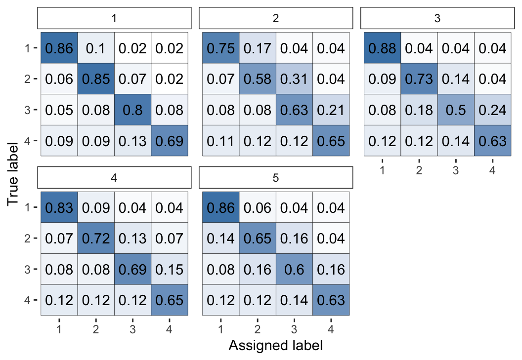
Figure 2: Visual representation of the inferred parameters in the error matrices (\(\theta\)) for the Dawid–Skene model fitted via MCMC to the anaesthesia dataset. The values shown are posterior means, with each cell shaded on a gradient from white (value close to 0) to dark blue (value close to 1).
We can see high values along the diagonals of these matrices, which indicates that each of the 5 anaesthetists is inferred as being fairly accurate at rating pre-operative health. Looking at the non-diagonal entries, we can see that typically the most common errors are 1-point differences on the rating scale.
The following command visualises the latent class probabilities, with the output shown in Figure 3:
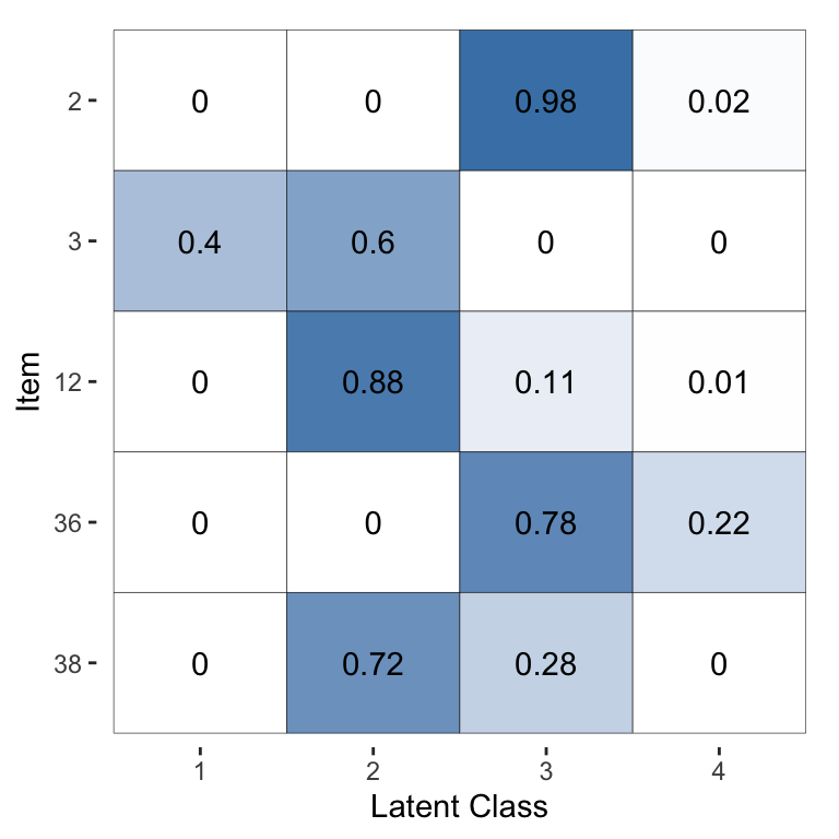
Figure 3: Visualisation of the inferred probability of each latent class, for a selected subset of items, for the Dawid–Skene model fitted via MCMC to the anaesthesia dataset.
For the purpose of illustration, for this plot we have selected the 5 patients with the greatest uncertainty in their pre-operative health (latent class). The other 40 patients all have almost no posterior uncertainty for their pre-operative health. Thus, suppose we wished to use the model to infer the pre-operative health by combining all of the anaesthetists’ ratings, we can do so confidently for all but a handful of patients.
The same output for the models fitted via
optimisation rather than MCMC (using fit_2 instead of fit_1) are
shown in Figure 4 and Figure 5. We can
see that this estimation method leads to the same broad conclusions, however the
optimisation-based estimates have considerably less uncertainty: they are
typically closer to 0 or 1. This behaviour reflects the fact that
optimisation-based inference will usually not capture the full uncertainty and
will lead to overconfident estimates. Thus, we recommend using MCMC (which we
have set as the default).
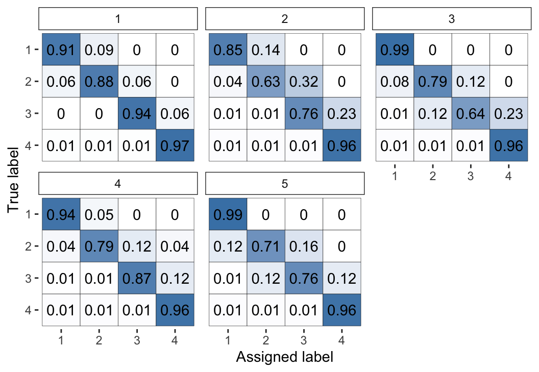
Figure 4: Visual representation of the inferred parameters in the error matrices (\(\theta\)) for the Dawid–Skene model fitted via optimisation to the anaesthesia dataset. Compare with Figure 2, which used MCMC instead of optimisation.
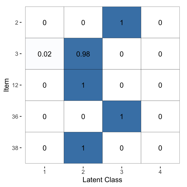
Figure 5: Visualisation of the inferred probability of each latent class, for a selected subset of items, for the Dawid–Skene model fitted via optimisation to the anaesthesia dataset. Compare with Figure 3, which used MCMC instead of optimisation.
While it is typically of less interest, it is also possible to visualise the prevalence estimates, together with credible intervals, using the following command (see output in Figure 6):
plot(fit_1, "prevalence")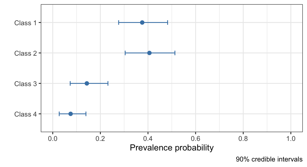
Figure 6: Visualisation of the inferred population prevalence parameters, with 90% credible intervals, for the Dawid–Skene model fitted to the anaesthesia dataset.
7.5 Different models and priors
The second argument to the rater() function specifies what model to use,
including details of the prior if not using the default one. This gives a
unified place to specify both the model and prior.
For example, this is how to set a different prior using the Dawid–Skene model:
diff_alpha_fit <- rater(anesthesia, dawid_skene(alpha = rep(10, 4)))When specifying the \(\beta\) hyper-parameters for the Dawid–Skene model, the user can either specify a single matrix or a 3-dimensional array. If only a matrix specified, it will be interpreted as the hyper-parameter values for all raters. This is useful in the common situation where the overall quality of the raters is known but there is no information on the quality of any specific rater. When a 3-dimensional array is passed, it is taken to specify the hyper-parameters for each of the raters (i.e., a separate matrix for each rater). This is useful when prior information about the quality of specific raters is available, for example when some ‘raters’ are diagnostic tests with known performance characteristics.
This is how to use the class-conditional Dawid–Skene model (with default prior):
diff_model_fit <- rater(anesthesia, class_conditional_dawid_skene())Compared with the Dawid–Skene model, the latter uses error matrices with the constraint that all off-diagonal entries must be the same. We can visualise the \(\theta\) parameter using the following command (output in Figure 7) and see that all off-diagonal elements are indeed equal:
plot(diff_model_fit, "theta")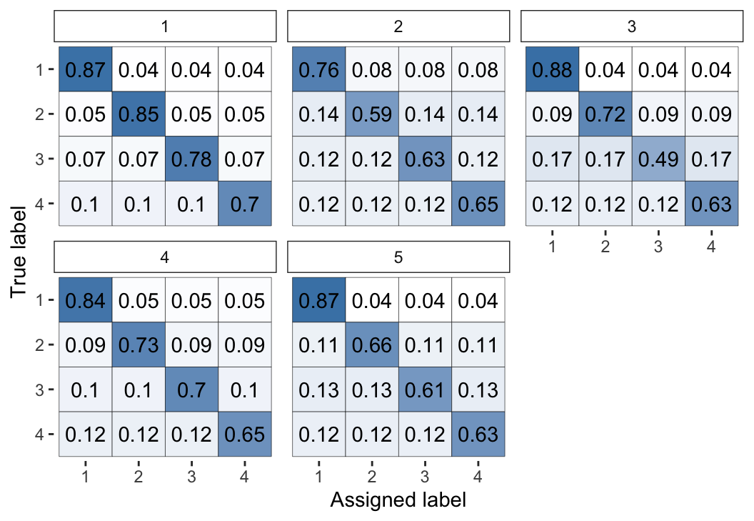
Figure 7: Visual representation of the inferred parameters in the error matrices (\(\theta\)) for the class-conditional Dawid–Skene model fitted via MCMC to the anaesthesia dataset. Compare with Figure 2, which used the standard Dawid–Skene model.
7.6 Using grouped data
The second example dataset is taken from Espeland and Handelman (1989). It consists of 3,689 binary ratings, made by 5 dentists, of whether a given tooth was healthy or had caries/cavities. The ratings were performed using X-ray only, which was thought to be more error-prone than visual/tactile assessment of each tooth (see Handelman et al. (1986) for more information and a description of the wider dataset from which these binary ratings were taken).
  rater_1 rater_2 rater_3 rater_4 rater_5    n
1       1       1       1       1       1 1880
2       1       1       1       1       2  789
3       1       1       1       2       1   43
4       1       1       1       2       2   75
5       1       1       2       1       1   23
6       1       1       2       1       2   63
This is an example of ‘grouped’ data. Each row represents a particular ratings ‘pattern’, with the final column being a tally that records how many instances of that pattern appear in the data. rater accepts data in either ‘long’, ‘wide’ or ‘grouped’ format. The ‘long’ format is the default because it can represent data with repeated ratings. When available the ‘grouped’ format can greatly speed up the computation of certain models and is convenient for datasets that are already recorded in that format. The ‘wide’ format doesn’t provide any computational advantages but is a common format for data without repeated ratings and so is provided for convenience.
Here’s how we fit the model to grouped data (note the data_format
argument):
fit3 <- rater(caries, dawid_skene(), data_format = "grouped")From there, we can inspect the model fit in the same way as before. For example (output shown in Figure 8):
plot(fit3, "raters")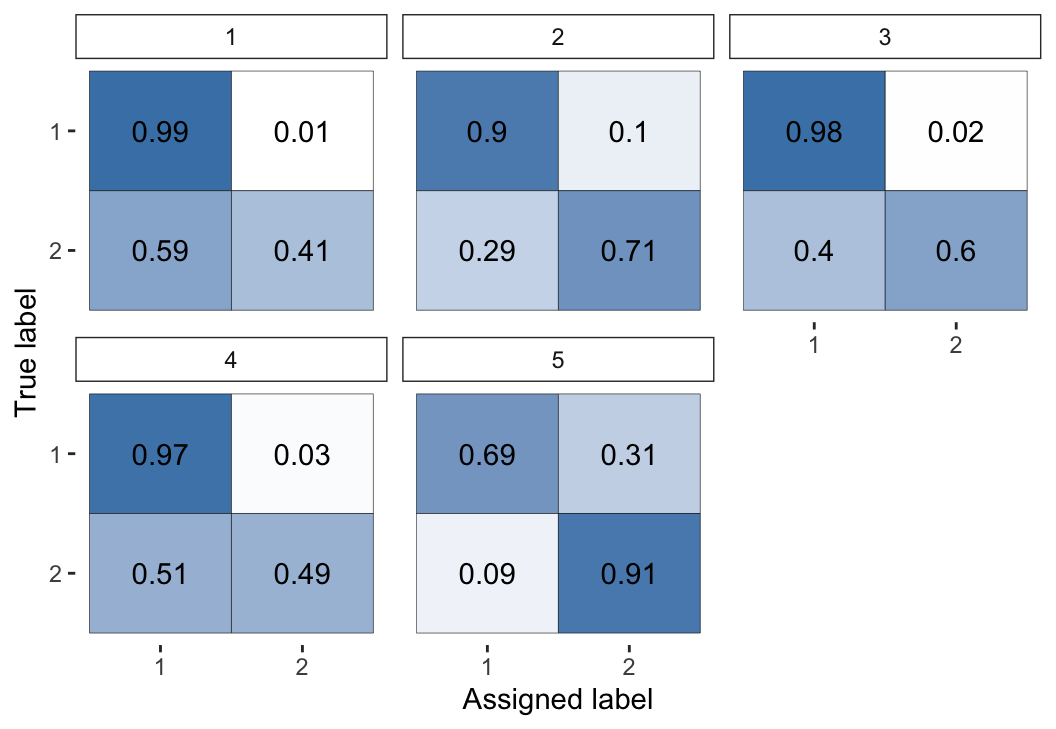
Figure 8: Visual representation of the inferred parameters in the error matrices (\(\theta\)) for the Dawid–Skene model fitted via MCMC to the caries dataset.
The first 4 dentists are highly accurate at diagnosing healthy teeth (rating \(= 1\)), but less so at diagnosing caries (rating \(= 2\)). In contrast, the 5th dentist was much better at diagnosing caries than healthy teeth.
7.7 Convergence diagnostics
A key part of applied Bayesian statistics is assessing whether the
MCMC sampler has converged on the posterior distribution. To summarise the
convergence of a model fit using MCMC, rater provides the
mcmc_diagnostics() function.
head(mcmc_diagnostics(fit_1)) Rhat ess_bulk
pi[1] 1.000309 8714.189
pi[2] 1.000377 8357.551
pi[3] 1.000275 8202.908
pi[4] 1.001472 7701.453
theta[1, 1, 1] 1.001018 8332.856
theta[1, 1, 2] 1.001445 8015.780This function calculates and displays the \(\hat{R}\) statistic (Rhat) and bulk
effective sample size (ess_bulk) for all of the \(\pi\) and \(\theta\)
parameters. Users can then check for the convergence of specific parameters by
applying standard rules, such as considering that convergence has been reached
for a specific parameter if it’s \(\hat{R} < 1.01\) (Vehtari et al. 2021).
Users wishing to calculate other metrics, or produce convergence visualisations
such as trace plots, can either extract the underlying Stan model from the
rater fit using the get_stanmodel() function, or convert the
fit into a mcmc.list from the coda package using the
as_mcmc.list() function. Functions in the rstan and
coda packages will then allow visualisation based assessment of
convergence and the calculation of other, more advanced, diagnostics.
For example, the following code uses rstan to draw the trace plot (shown in Figure 9) for one of the parameters from the Dawid–Skene model fitted to the anaesthesia data. We can see that the four chains show good mixing. The trace plots for the other parameters (not shown here) are similar, indicating that the MCMC sampling procedure has converged.
stan_fit <- get_stanfit(fit_1)
rstan::traceplot(stan_fit, pars = "pi[1]")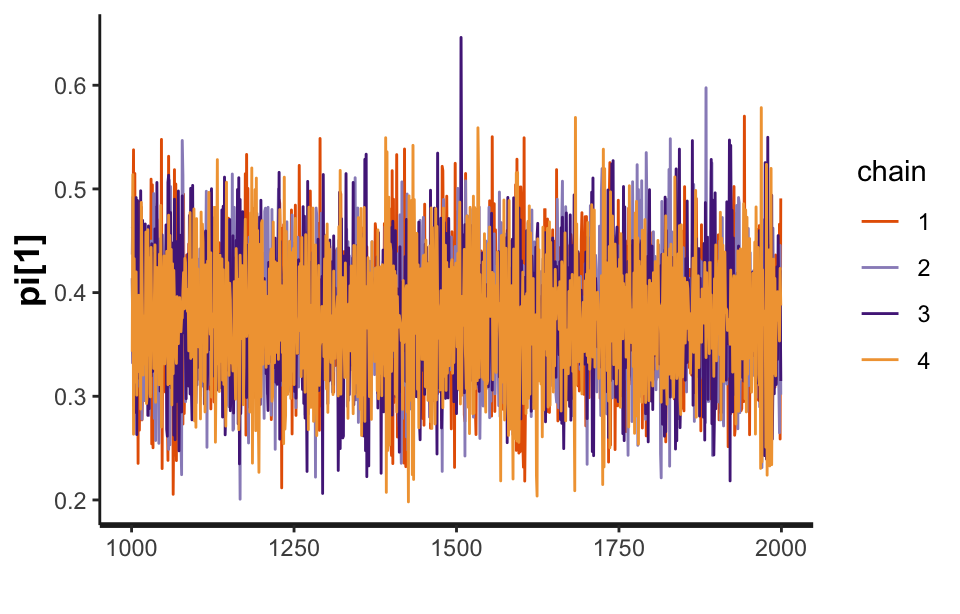
Figure 9: A trace plot for the \(\pi_1\) parameter from the Dawid–Skene model fitted via MCMC to the anaesthesia dataset.
7.8 Model assessment and comparison
Finally, rater provides facilities to assess and compare fitted
models. First, it provides the posterior_predict() function to simulate from
the posterior predictive distributions of all the models implemented in
rater. The simulated data can then be used, for example, to perform
posterior predictive checks. These checks compare the data
simulated from the fitted model to the observed data. A number of datasets
are simulated from the posterior predictive distribution and a summary statistic
is calculated for each dataset. The same summary statistic is calculated on the
observed dataset and is compared to the distribution of simulated statistics.
A large discrepancy between the simulated statistics and the observed statistic
indicates possible model misspecification.
To illustrate this functionality, we consider assessing the fit of the Dawid–Skene model to the anaesthesia dataset. In this example, we simulate 1,000 datasets from the posterior predictive distribution, and use the proportion of the ratings that are class 2 as a statistic to summarise each dataset.
class2prop <- function() {
  simdata <- posterior_predict(fit_1, anesthesia[, 1:2])
  sum(simdata$rating == 2) / nrow(simdata)
}
ppc_statistics <- replicate(1000, class2prop())
head(ppc_statistics)
[1] 0.3079365 0.3333333 0.4158730 0.2666667 0.2793651 0.3587302We can then graphically compare the distribution of these statistics to the value of the same statistic applied to the anaesthesia dataset. The following commands will create such a plot (shown in Figure 10):
ggplot(data.frame(prop_class_two = ppc_statistics), aes(prop_class_two)) +
  geom_histogram(binwidth = 0.01, fill = "steelblue", colour = "black") +
  geom_vline(xintercept = sum(anesthesia$rating == 2) / nrow(anesthesia),
             colour = "black", linewidth = 2) +
  theme_bw() +
  coord_cartesian(xlim = c(0.1, 0.6)) +
  labs(
    x = "Proportion of class 2 ratings",
    y = "Count"
  )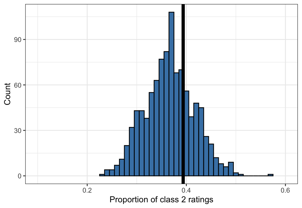
Figure 10: An example of a posterior predictive check for the Dawid–Skene model fitted via MCMC to the anaesthesia dataset. Shown is a histogram of 1,000 simulated datasets from the posterior predictive distribution, each summarised by the proportion of ratings that are class 2. The vertical black line shows the proportion of ratings that are class 2 in the original dataset, for comparison against the histogram.
The statistic calculated on the anaesthesia dataset lies towards the centre of the distribution of statistics calculated from datasets drawn from the posterior predictive distribution. This is consistent with the model fitting the data well. (This is an illustrative example only. A more comprehensive set of such comparisons should be conducted before concluding that the model adequately describes the data.)
Second, rater implements the functions loo() and waic()
to provide model comparison metrics using the loo package. The
function loo() calculates an approximation to leave-out-one
cross-validation, a measure of model performance using Pareto Smoothed
Importance Sampling (Vehtari et al. 2017). The function waic() calculates
measures related to the Widely Applicable Information Criterion
(Watanabe 2013). Because rater fits models in a Bayesian
framework, information criteria such as the AIC and BIC are not implemented.
In the context of rater, model comparison is only possible between
the different implemented models, not between the same model with different
parameter values or included covariates, as is more commonly the case. For
this reason, considerations of data size and what is known about the
characteristics of the raters should also be taken into account when making
such choices, in addition to the output of loo() and waic().
To briefly illustrate some of this functionality, we compare the standard Dawid–Skene model to the class-conditional one.
loo(fit_1)
Computed from 4000 by 45 log-likelihood matrix

         Estimate   SE
elpd_loo   -234.0 17.0
p_loo        20.2  2.7
looic       468.0 34.0
------
Monte Carlo SE of elpd_loo is 0.1.

Pareto k diagnostic values:
                         Count Pct.    Min. n_eff
(-Inf, 0.5]   (good)     39    86.7%   677
 (0.5, 0.7]   (ok)        6    13.3%   407
   (0.7, 1]   (bad)       0     0.0%   <NA>
   (1, Inf)   (very bad)  0     0.0%   <NA>

All Pareto k estimates are ok (k < 0.7).
See help('pareto-k-diagnostic') for details.loo(diff_model_fit)
Computed from 4000 by 45 log-likelihood matrix

         Estimate   SE
elpd_loo   -245.7 18.1
p_loo        10.2  1.2
looic       491.3 36.1
------
Monte Carlo SE of elpd_loo is 0.1.

All Pareto k estimates are good (k < 0.5).
See help('pareto-k-diagnostic') for details.loo_compare(loo(fit_1), loo(diff_model_fit)) elpd_diff se_diff
model1 0.0 0.0
model2 -11.7 3.2 From these results, we see that both models fit the data well, with the class-conditional model being slightly preferred.
8 Summary and discussion
Rating procedures, in which items are sorted into categories, are subject to both classification error and uncertainty when the categories themselves are defined subjectively. Data that results from these types of tasks require a proper statistical treatment if: (1) the population frequencies of the categories are to be estimated with low bias, (2) items are to be assigned to these categories reliably, and (3) the agreement of raters is to be assessed. To date there have been few options for practitioners seeking software that implements the required range of statistical models. The R package described in this paper, rater, provides the ability to fit Bayesian versions of a variety of statistical models to categorical rating data, with a range of tools to extract and visualise parameter estimates.
The statistical models that we have presented are based on the Dawid–Skene model and recent modifications of it including extensions, such as the hierarchical Dawid–Skene model where the rater-specific parameters are assumed to be drawn from a population distribution, and simplifications that, for example, assume exchangeable raters with identical performance characteristics (homogeneous Dawid–Skene), or homogeneity criteria where classification probabilities are identical regardless of the true, underlying category of an item (class-conditional Dawid–Skene).
We provided: (1) an explanation of the type of data formats that categorical ratings are recorded in, (2) a description of the construction and implementation of the package, (3) a comparison of our package to other existing packages for fitting latent class models in R, (4) an introduction to the user interface, and (5) worked examples of real-world data analysis using rater.
We devoted an entire section to motivating, deriving and explaining the use of a marginalised version of the joint posterior probability distribution to remove dependence on the unknown value of the true, underlying rating category of an item. This is necessary because the No-U-Turn Sampler, the main MCMC algorithm used in Stan, relies on computing derivatives with respect to all parameters that must, therefore, be continuously-valued. The technique involves the use of conditional expectation and is a special case of a more general technique of conditioning or ‘Rao–Blackwellization’, the process of transforming an estimator using the Rao–Blackwell theorem to improve its efficiency.
Our package was developed with the classification of medical images in mind, where there may be a large number of images but typically only a small number of possible categories and a limited number of expert raters. The techniques proposed based on extensions of the Dawid–Skene model readily extend to scenarios where the datasets are much larger, or where the raters behave erratically (cannot be relied on to rate correctly more frequently than they rate incorrectly) or are antagonistic (deliberately attempt to allocate items to a category not favoured by the majority of raters).
One possible extension of the Dawid–Skene model is to add item- and rater-specific covariates. These covariates would encode the difficulty of items and the expertise (or lack thereof) of the raters. This extension is particularly attractive as it would partially alleviate the strong assumption of independence conditional on the latent class, replacing it with the weaker assumption of independence conditional on the latent class and the covariates. Unfortunately, these types of models would contain many more parameters than the original Dawid–Skene model making them difficult to fit, especially when used with relatively small datasets common in the context of rating data in medical research. Therefore, future methodological research is needed before these models can be included in the rater package. Latent class models with covariates can be fitted, although only in a frequentist framework, using the R package poLCA.
9 Computational details
The results in this paper were obtained using R 4.2.2 (R Core Team 2021) and the following packages: coda 0.19.4 (Plummer et al. 2006), ggplot2 3.4.3 (Wickham 2016), knitr 1.45 (Xie 2014, 2015, 2023), loo 2.6.0 (Vehtari et al. 2023), rater 1.3.1 (Pullin and Vukcevic 2023), rjtools 1.0.12 (O’Hara-Wild et al. 2023), rmarkdown 1.0.12 (Xie et al. 2018, 2020; Allaire et al. 2023), rstan 2.26.23 (Stan Development Team 2023). R itself and all packages used are available from the Comprehensive R Archive Network (CRAN).
10 Acknowledgments
We would like to thank Bob Carpenter for many helpful suggestions, and David Whitelaw for his flexibility in allowing the first author to work on this paper while employed at the Australian Institute of Heath and Welfare. Thanks also to Lars Mølgaard Saxhaug for his code contributions to rater.
10.1 Supplementary materials
Supplementary materials are available in addition to this article. It can be downloaded at RJ-2023-064.zip
10.2 CRAN packages used
rater, poLCA, BayesLCA, randomLCA, coda, rstan, loo, ggplot2, knitr, rjtools, rmarkdown
10.3 CRAN Task Views implied by cited packages
Bayesian, Cluster, GraphicalModels, MixedModels, Phylogenetics, Psychometrics, ReproducibleResearch, Spatial, TeachingStatistics